Efficient Similarity Search with FAISS
FAISS (Facebook AI Similarity Search) is a high-performance library that expedites similarity search and classification, consuming high-dimensional vectors derived from cutting-edge AI tools such as word2vec or Convolutional Neural Networks (CNN). This article gives a brief introduction about how to use it efficiently, especially with PySpark.
TL;DR: To obtain maximal performance gains, search with a batch of queries rather than a single one.
Getting Started: A Minimal Working Example
Prior to diving into the examples, it is imperative that FAISS is installed. It’s highly advised to install FAISS via conda, as opposed to PyPI, to circumvent potential compatibility issues.
Assuming the availability of FAISS, we can go through an MWE to understand its basic functionality.
import faiss

import numpy as np
from typing import Tuple

def get_index(vectors: np.ndarray) -> faiss.IndexFlatL2:
    # build the index
    index = faiss.IndexFlatL2(vectors.shape[1])
    # add vectors to the index
    index.add(vectors.astype(np.float32))
    return index

def search(
    index: faiss.IndexFlatL2, query: np.ndarray, k: int
) -> Tuple[np.ndarray, np.ndarray]:
    # search the k nearest neighbors of query in the index
    return index.search(query, k)

# construct a n * d (5 * 3) numpy matrix of type float32
all_vectors = np.array(
    [[1, 2, 3], [4, 5, 6], [7, 8, 9], [10, 11, 12], [13, 14, 15]], dtype=np.float32
)

# define a m * d (1 * 3) matrix with query vectors
single_query = np.array([[9, 10, 11]], dtype=np.float32)

index = get_index(all_vectors)
result = search(index, single_query, 5)

print(result)

# output
"""
(array([[  3.,  12.,  48.,  75., 192.]], dtype=float32), array([[3, 2, 4, 1, 0]]))
"""
Initially, we build an IndexFlatL2 object, which employs a brute-force algorithm for similarity searches based on Euclidean distances. Subsequently, we add some concrete vectors to the index and perform a similarity search. The search method returns a tuple of numpy.ndarrays, with two elements representing the L2 distances and the sequential ids respectively, of up to k vectors closest to the query vector.
FAISS is fully integrated with NumPy, and thus all functions accept NumPy arrays as input. It is crucial to highlight that FAISS does not support double precision floating-point format so all numpy.ndarrays must be of numpy.float32.
With an understanding of how it works, a concise function can be extracted:
def get_k_nearest(vectors: np.ndarray, query: np.ndarray, k: int):
    index = faiss.IndexFlatL2(vectors.shape[1])
    index.add(vectors.astype(np.float32))
    return index.search(query, k)
Although this function is less likely to be used in a production environment due to the fact that searching is generally more frequent than building indexes, it illustrates the foundational operations within FAISS:
- Build an index, specifying the dimensionality of the vectors it will operate on
- Add elements to the index
- (Optional) Train to analyze the distribution of the vectors
- Execute search operations on the index
Faster Search with PySpark
A quintessential application of FAISS is to perform similarity searches among a vast collection of items. Suppose there are millions of items, and we would like to find the top 100 most similar items for each of them. It is not ideal to handle such a volume of data on a single node, so we use PySpark to parallelize this process. The following shows the primary part of the legacy production code.
def findNeighbors(partitionData):
    index = faiss.read_index(SparkFiles.get(faiss_model_name))
    for row in partitionData:
        item_id = row.item_id
        vector = np.array(row.embedding).reshape(1, -1).astype("float32")
        _, I = index.search(vector, topK + 1)
        sim_items = vectors.loc[I[0]]["item_id"].tolist()[1:]
        yield [item_id, sim_items]


if __name__ == "__main__":
    # load data from Hive table to Spark Dataframe
    # for each item, there is a unique id and an array of embeddings reflecting its feature
    sql = f"""
        select
            item_id
            , embedding
        from
            {item_embedding_table}
        where
            partition_date = '{partition_date}'
            and partition_region = '{partition_region}'
            and queue = '{model_name}'
    """
    item_emb = spark.sql(sql)

    # collect the data and normalize
    vectors = item_emb.toPandas()
    print(vectors.shape)
    vectors["embedding"] = vectors["embedding"].apply(np.array)

    # build the index and add vectors to the index
    index = faiss.IndexFlatL2(emb_size)
    print(index.is_trained)
    index.add(np.array(vectors["embedding"].tolist()).astype("float32"))

    # dump index to disk and distribute the file
    faiss_model_name = f"faiss_{partition_region}_{model_name}.model"
    faiss.write_index(index, faiss_model_name)
    sc.addPyFile(faiss_model_name)

    # item ids are required to map from sequential ids
    vectors.columns = ["item_id", "embedding"]
    vectors = vectors[["item_id"]]

    i2i = (
        item_emb.rdd.repartition(i2i_repartition_num[partition_region])
        .mapPartitions(findNeighbors)
        .toDF(["item_id", "sim_item_id"])
        .select("item_id", F.posexplode("sim_item_id"))
        .withColumn("score", (lit(topK) - col("pos")) / lit(topK))
        .withColumnRenamed("col", "sim_item_id")
        .select(
            col("item_id").cast("bigint"),
            col("sim_item_id").cast("bigint"),
            col("score").cast("double"),
        )
    )

    # function implementation is omitted
    save2Hive(
        partition_date,
        partition_region,
        i2i,
        i2i_table,
        model_name,
        i2i_save_partition_num[partition_region],
    )
Pinpointing the Bottleneck: A Quick Diagnosis
While the underlying business logic is straightforward, the Spark job took more than 7 hours to calculate similarity across approximately 9.6 million items. How to make it faster? We need to take a closer look at the findNeighbors function.
def findNeighbors(partitionData):
    # download the index file and load it into memory on each node
    index = faiss.read_index(SparkFiles.get(faiss_model_name))

    # iterate over partitioned data
    for row in partitionData:
        # get item id, which will be returned subsequently as it is
        item_id = row.item_id
        # get embedding representing the current item
        vector = np.array(row.embedding).reshape(1, -1).astype("float32")
        # get sequential ids of the top K + 1 most similar items
        # why K + 1 instead of K: the query vector is one of the vectors in index
        _, I = index.search(vector, topK + 1)
        # get the corresponding item id from the sequential id
        sim_items = vectors.loc[I[0]]["item_id"].tolist()[1:]
        yield [item_id, sim_items]
In this case, mapPartitions is favored over map as it diminishes the frequency of index loading, transitioning from once per record to once per partition. We can further optimize it with the help of broadcast variables. Having said that, the QPS of the search method of faiss.IndexFlatL2 remains the biggest possible performance bottleneck of the Spark job. Although the documentation states that queries should be submitted by batches to obtain the best performance, it might not be intuitively evident how to implement this.
Harnessing the Power of Batch Processing
Actually, insights can be drawn from the MWE discussed earlier. Notably, both all_vectors and single_query are x * d NumPy matricex (i.e. they must have the same shape[1] but may have different shape[0]). Instinctively, we can convert a single query to multiple queries.
multiple_queries = np.array([[9, 10, 11], [4, 5, 6], [1000, 100, 10]], dtype=np.float32)

print(search(get_index(all_vectors), multiple_queries, 5))

# output
"""
(array([[3.000000e+00, 1.200000e+01, 4.800000e+01, 7.500000e+01,
         1.920000e+02],
        [0.000000e+00, 2.700000e+01, 2.700000e+01, 1.080000e+02,
         2.430000e+02],
        [9.815900e+05, 9.880250e+05, 9.945140e+05, 1.001057e+06,
         1.007654e+06]], dtype=float32),
 array([[3, 2, 4, 1, 0],
        [1, 2, 0, 3, 4],
        [4, 3, 2, 1, 0]]))
"""
As the output shows, batch searches can be executed by merely converting a single query into multiple queries without altering the search method. With this knowledge, refactoring the findNeighbors function becomes feasible.
# ... context is omitted
broadcasted_vectors = sc.broadcast(vectors)
broadcasted_index = sc.broadcast(index)
# ...


def find_neighbors(partition_data):
    b_index = broadcasted_index.value
    b_vectors = broadcasted_vectors.value

    _iterator = []

    multiple_vectors = None

    item_ids = []

    for row in partition_data:
        item_ids.append(row.item_id)
        vector = np.array(row.embedding).reshape(1, -1).astype("float32")

        multiple_vectors = (
            np.append(multiple_vectors, vector, axis=0)
            if multiple_vectors is not None
            else vector
        )

    # use batch search instead of single search
    _, I = b_index.search(multiple_vectors, topK + 1)

    for _id, each in enumerate(I):
        _iterator.append([item_ids[_id], b_vectors.loc[each]["item_id"].tolist()[1:]])

    return iter(_iterator)
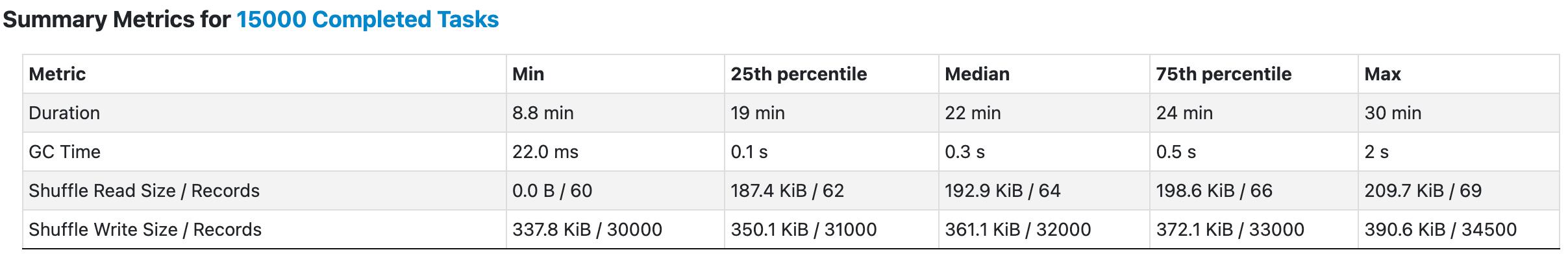
The simple idea is to alleviate the data loading overhead by broadcasting both indexes and queries, and perform only one search for each partition as a batch. In this way, we can easily control the number of records within a single batch by employing repartition. This enhancement has yielded remarkable gains: the search speed has improved tenfold.
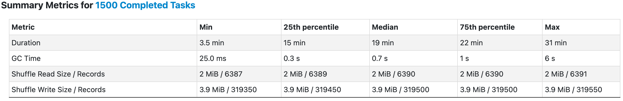
It is pertinent to mention that the number of repartitions was intentionally reduced to one-tenth of the original number. Contrary to what one might assume, increasing the number of partitions indefinitely is not necessarily beneficial. In fact, an excessive number of partitions can introduce additional overhead and occasionally give rise to tricky issues. A carefully considered partition strategy is essential for both good performance and resource utilization.
Exploiting Vectorization with Numpy
Moreover, we can further leverage NumPy native features to benefit from inherent SIMD optimizations, or simply make the functions more compact. The following version gains slight but definite performance improvements over the previous one.
def compact_find_neighbors(partition_data):
    b_index = broadcasted_index.value
    b_vectors = broadcasted_vectors.value

    item_ids, multiple_vectors = zip(
        *(
            (row.item_id, np.array(row.embedding).reshape(1, -1).astype("float32"))
            for row in partition_data
        )
    )

    # use batch search instead of single search
    _, I = b_index.search(np.concatenate(list(multiple_vectors)), topK + 1)

    return (
        (item_id.item(0), b_vectors["item_id"].values[sim_item_id[1:]].tolist())
        for item_id, sim_item_id in np.nditer(
            [np.concatenate([[e] for e in item_ids]).reshape(-1, 1), I],
            flags=["external_loop"],
        )
    )
Based on the C++ API documentation, we have the option to substitute the search function with assign if we only need the labels of neighbors without specific distances.
def piped_find_neighbors(partition_data):
    return (
        (item_id.item(0), broadcasted_vectors.value["item_id"].values[sim_item_id[1:]].tolist())
        for item_id, sim_item_id in np.nditer(
            list(
                *(
                    (
                        np.concatenate([[_id] for _id in item_ids]).reshape(-1, 1),
                        broadcasted_index.value.assign(
                            np.concatenate(list(multiple_vectors)), topK + 1
                        ),
                    )
                    for (item_ids, multiple_vectors) in (
                        (
                            v
                            for v in zip(
                                *(
                                    (
                                        _row.item_id,
                                        np.array(_row.embedding)
                                        .reshape(1, -1)
                                        .astype("float32"),
                                    )
                                    for _row in partition_data
                                )
                            )
                        ),
                    )
                )
            ),
            flags=["external_loop"],
        )
    )
While this version curtails potential memory consumption, it comes at the expense of readability, which may render it suboptimal in numerous scenarios. Merely with the first refactored version find_neighbors, the average execution time of the Spark job has been reduced to around one-ninth of the original. Of course, several additional advanced features of Spark have been adopted as well during this process, which won’t be covered in this article.
Upholding Code Integrity: Regression Testing
Prior to deploying the optimized code to the production environment, it is imperative to conduct regression testing to ascertain that the modifications do not adversely impact the existing functionalities. Comprehensive regression testing encompasses multiple facets and intricate logic. For illustrative purposes, a simplified version of regression testing is showcased below:
-- Presto SQL

with
    prod_table as
    (
        select
            *
        from
            some_db.prodction_table
        where
            partition_region = 'SG' and partition_date = '2023-01-02'
    ),

    test_table as
    (
        select
            *
        from
            some_db.testing_table
        where
            partition_region = 'SG' and partition_date = '2023-01-02'
    ),

    union_table as
    (
        select * from prod_table

        union

        select * from test_table
    ),

    intersection_table as
    (
        select * from prod_table

        intersect

        select * from test_table
    )

select
    (select count(*) from prod_table) = (select count(*) from test_table) as records_num_not_change,
    (
        (select count(*) from union_table) - (select count(*) from intersection_table)
    )
    /
    (select cast(count(*) as double) from union_table) * 100 as records_not_match_percentage

-- output
/*
    records_num_not_change  |   records_not_match_percentage
    true                    |   0.11059705816904215
*/
Surprisingly, the outcome reveals that about 0.11% of the records do not align. Then we need to discern the specific discrepancies.
-- same `with` clause in CTE as above is omitted

select
    *
from
    union_table
except
    (
        select
            *
        from
            intersection_table
    )
order by
    item_id
    ,sim_item_id
limit
    20

-- output is omitted
Specifically, it emerges that batch searches may sporadically interchange the order of, for example, the 45th and 46th elements in a 50-element sorting compared to single searches. This discrepancy can be attributed to the implementation of the L2 distance computation in FAISS, which, due to the limited precision of float32, can result in catastrophic cancellation in some cases . No known practical workaround has been found for this issue, but there is no need to solve it either. As stated, FAISS is primarily tailored for high-performance searches, and as such, most indexes are approximate in nature.
Additional Resources
- Wiki
- Engineering Blog
- C++ API Documentation
- Johnson, Jeff, Matthijs Douze, and Hervé Jégou. “Billion-scale similarity search with gpus.” IEEE Transactions on Big Data 7.3 (2019): 535-547.
This article is based on Python 3.6.13 and faiss-cpu 1.7.1.